聚类算法综述

文章目录

1. 1. 常见聚类算法
   1. 1.1. K均值（Kmeans）
   2. 1.2. 均值漂移（Mean Shift）
   3. 1.3. DBSCAN
   4. 1.4. 高斯混合模型
   5. 1.5. 凝聚层次聚类
2. 2. sklearn实现
3. 3. 参考

聚类是机器学习中一种重要的无监督算法，它试图将数据集中的样本划分为若干个通常不相交的子集，每个子集成为一个“簇”（cluster），理论上来说，每一簇对应一个潜在的概念，但这个概念事先并不知道，需要使用者来把握。本文是常见聚类算法的综述，为了加深理解，大部分算法配有动图。

常见聚类算法

K均值（Kmeans）

这一最著名的聚类算法，主要基于数据点之间的均值和与聚类中心的聚类迭代而成。它主要的优点是十分的高效，由于只需要计算数据点与聚类中心的距离，其计算复杂度只有O(n)。

1.首先我们需要预先给定聚类的数目同时随机初始化聚类中心。我们可以粗略的观察数据并给出较为准确的聚类数目；
2.每一个数据点通过计算与聚类中心的距离了来分类到最邻近的一类中；
3.根据分类结果，利用分类后的数据点重新计算聚类中心；
4.重复步骤2、3直到聚类中心不再变化。（可以随机初始化不同的聚类中心以选取最好的结果）

这种方法在理解和实现上都十分简单，但缺点却也非常明显：十分依赖于初始给定的聚类数目；同时随机初始化可能会生成不同的聚类效果，所以它缺乏重复性和连续性。
和K均值类似的K中值算法，在计算过程中利用中值来计算聚类中心，使得局外点对它的影响大大减弱；但每一次循环计算中值矢量带来了计算速度的大大下降。

均值漂移（Mean Shift）

这是一种基于滑动窗口的均值算法，用于寻找数据点中密度最大的区域。其目标是找出每一个类的中心点，并通过计算滑窗内点的均值更新滑窗的中心点。最终消除临近重复值的影响并形成中心点，找到其对应的类别。

1.首先，以随机选取的点为圆心，r为半径做一个圆形的滑窗。其目标是找出数据点中密度最高点并作为中心；
2.在每个迭代后，滑动窗口的中心将向较高密度的方向移动；
3.连续移动，直到任何方向的移动都不能增加滑窗中点的数量，此时滑窗收敛；
4.将上述步骤在多个滑窗上进行以覆盖所有的点。当多个滑窗收敛重叠时，其经过的点将会通过其滑窗聚类为一个类。

下图中每一个黑点都代表一个滑窗的中心，他们最终重叠在每一类的中心；

与K均值相比最大的优点是，我们无需指定指定聚类数目，聚类中心处于最高密度处也是符合直觉认知的结果。但其最大的缺点在于滑窗大小r的选取，对于结果有着很大的影响。

DBSCAN

DBSCAN同样是基于密度的聚类算法，但其原理却与均值漂移大不相同：

1.首先从没有被遍历的任一点开始，利用邻域距离epsilon来获取周围点；
2.如果邻域内点的数量满足阈值则此点成为核心点并以此开始新一类的聚类。（如果不是则标记为噪声）；
3.其邻域内的所有点也属于同一类，将所有的邻域内点以epsilon为半径进行步骤2的计算；
4.重复步骤2、3直到遍历完所有核心点的邻域点；
5.此类聚类完成，同时又以任意未遍历点开始步骤1到4直到所有数据点都被处理；
6.最终每个数据点都有自己的归属类别或者属于噪声。

这种方法最大的优点在于无需定义类的数量，其次可以识别出局外点和噪声点，并且可以对任意形状的数据进行聚类。
但也存在不可回避的缺点，当数据密度变化剧烈时，不同类别的密度阈值点和领域半径会产生很大的变化。同时在高维空间中准确估计领域半径也是不小的挑战。

高斯混合模型

通过假设数据点符合均值和标准差描述的高斯混合模型来实现的。下图以二维情况下为例描述了如何利用最大期望优化算法来获取分布参数的过程：

1.首先确定聚类的数量，并随机初始化每一个聚类的高斯分布参数；
2.通过计算每一个点属于高斯分布的概率来进行聚类。与高斯中心越近的点越有可能属于这个类；
3.基于上一步数据点的概率权重，通过最大似然估计的方法计算出每一类数据点最有可能属于这一聚类的高斯参数；
4.基于新的高斯参数，重新估计每一点归属各类的概率，重复2，3步骤直到参数不再变化收敛为止。

在使用高斯混合模型时有两个关键的地方，首先高斯混合模型十分灵活，可以拟合任意形状的椭圆；其次这是一种基于概率的算法，每个点可以拥有属于多类的概率，支持混合属性。

凝聚层次聚类

层次聚类法主要有自顶向下和自底向上两种方式。其中自底向上的方式，最初将每个点看做是独立的类别，随后通过一步步的凝聚最后形成独立的一大类，并包含所有的数据点。这会形成一个树形结构，并在这一过程中形成聚类。

1.首先将每一个数据点看成一个类别，通过计算点与点之间的距离将距离近的点归为一个子类，作为下一次聚类的基础；
2.每一次迭代将两个元素聚类成一个，上述的子类中距离最近的两两又合并为新的子类。最相近的都被合并在一起；
3.重复步骤2直到所有的类别都合并为一个根节点。基于此我们可以选择聚类的数目，并根据树来进行选择。

层次聚类无需事先指定类的数目，并且对于距离的度量不敏感。这种方法最好的应用在于恢复出数据的层次化结构。但其计算复杂度较高达到了O（n^3）.

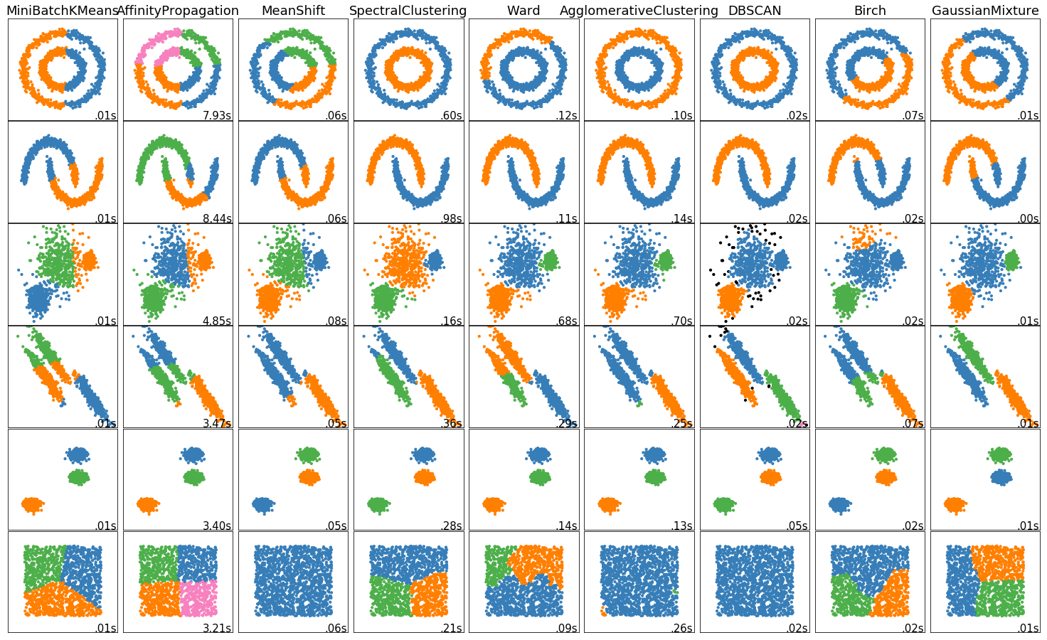
sklearn实现

sklearn官网(http://scikit-learn.org/stable/modules/clustering.html#clustering) 对常见的聚类算法做了汇总比较，结果一目了然，可以看出DBSCAN在训练时长和结果上均有优异表现，最终效果如下：

实现代码如下：

import time
import warnings

import numpy as np
import matplotlib.pyplot as plt

from sklearn import cluster, datasets, mixture
from sklearn.neighbors import kneighbors_graph
from sklearn.preprocessing import StandardScaler
from itertools import cycle, islice

np.random.seed(0)

# ============
# Generate datasets. We choose the size big enough to see the scalability
# of the algorithms, but not too big to avoid too long running times
# ============
n_samples = 1500
noisy_circles = datasets.make_circles(n_samples=n_samples, factor=.5,
                                      noise=.05)
noisy_moons = datasets.make_moons(n_samples=n_samples, noise=.05)
blobs = datasets.make_blobs(n_samples=n_samples, random_state=8)
no_structure = np.random.rand(n_samples, 2), None

# Anisotropicly distributed data
random_state = 170
X, y = datasets.make_blobs(n_samples=n_samples, random_state=random_state)
transformation = [[0.6, -0.6], [-0.4, 0.8]]
X_aniso = np.dot(X, transformation)
aniso = (X_aniso, y)

# blobs with varied variances
varied = datasets.make_blobs(n_samples=n_samples,
                             cluster_std=[1.0, 2.5, 0.5],
                             random_state=random_state)

# ============
# Set up cluster parameters
# ============
plt.figure(figsize=(9 * 2 + 3, 12.5))
plt.subplots_adjust(left=.02, right=.98, bottom=.001, top=.96, wspace=.05,
                    hspace=.01)

plot_num = 1

default_base = {'quantile': .3,
                'eps': .3,
                'damping': .9,
                'preference': -200,
                'n_neighbors': 10,
                'n_clusters': 3}

datasets = [
    (noisy_circles, {'damping': .77, 'preference': -240,
                     'quantile': .2, 'n_clusters': 2}),
    (noisy_moons, {'damping': .75, 'preference': -220, 'n_clusters': 2}),
    (varied, {'eps': .18, 'n_neighbors': 2}),
    (aniso, {'eps': .15, 'n_neighbors': 2}),
    (blobs, {}),
    (no_structure, {})]

for i_dataset, (dataset, algo_params) in enumerate(datasets):
    # update parameters with dataset-specific values
    params = default_base.copy()
    params.update(algo_params)

    X, y = dataset

    # normalize dataset for easier parameter selection
    X = StandardScaler().fit_transform(X)

    # estimate bandwidth for mean shift
    bandwidth = cluster.estimate_bandwidth(X, quantile=params['quantile'])

    # connectivity matrix for structured Ward
    connectivity = kneighbors_graph(
        X, n_neighbors=params['n_neighbors'], include_self=False)
    # make connectivity symmetric
    connectivity = 0.5 * (connectivity + connectivity.T)

    # ============
    # Create cluster objects
    # ============
    ms = cluster.MeanShift(bandwidth=bandwidth, bin_seeding=True)
    two_means = cluster.MiniBatchKMeans(n_clusters=params['n_clusters'])
    ward = cluster.AgglomerativeClustering(
        n_clusters=params['n_clusters'], linkage='ward',
        connectivity=connectivity)
    spectral = cluster.SpectralClustering(
        n_clusters=params['n_clusters'], eigen_solver='arpack',
        affinity="nearest_neighbors")
    dbscan = cluster.DBSCAN(eps=params['eps'])
    affinity_propagation = cluster.AffinityPropagation(
        damping=params['damping'], preference=params['preference'])
    average_linkage = cluster.AgglomerativeClustering(
        linkage="average", affinity="cityblock",
        n_clusters=params['n_clusters'], connectivity=connectivity)
    birch = cluster.Birch(n_clusters=params['n_clusters'])
    gmm = mixture.GaussianMixture(
        n_components=params['n_clusters'], covariance_type='full')

    clustering_algorithms = (
        ('MiniBatchKMeans', two_means),
        ('AffinityPropagation', affinity_propagation),
        ('MeanShift', ms),
        ('SpectralClustering', spectral),
        ('Ward', ward),
        ('AgglomerativeClustering', average_linkage),
        ('DBSCAN', dbscan),
        ('Birch', birch),
        ('GaussianMixture', gmm)
    )

    for name, algorithm in clustering_algorithms:
        t0 = time.time()

        # catch warnings related to kneighbors_graph
        with warnings.catch_warnings():
            warnings.filterwarnings(
                "ignore",
                message="the number of connected components of the " +
                "connectivity matrix is [0-9]{1,2}" +
                " > 1. Completing it to avoid stopping the tree early.",
                category=UserWarning)
            warnings.filterwarnings(
                "ignore",
                message="Graph is not fully connected, spectral embedding" +
                " may not work as expected.",
                category=UserWarning)
            algorithm.fit(X)

        t1 = time.time()
        if hasattr(algorithm, 'labels_'):
            y_pred = algorithm.labels_.astype(np.int)
        else:
            y_pred = algorithm.predict(X)

        plt.subplot(len(datasets), len(clustering_algorithms), plot_num)
        if i_dataset == 0:
            plt.title(name, size=18)

        colors = np.array(list(islice(cycle(['#377eb8', '#ff7f00', '#4daf4a',
                                             '#f781bf', '#a65628', '#984ea3',
                                             '#999999', '#e41a1c', '#dede00']),
                                      int(max(y_pred) + 1))))
        # add black color for outliers (if any)
        colors = np.append(colors, ["#000000"])
        plt.scatter(X[:, 0], X[:, 1], s=10, color=colors[y_pred])

        plt.xlim(-2.5, 2.5)
        plt.ylim(-2.5, 2.5)
        plt.xticks(())
        plt.yticks(())
        plt.text(.99, .01, ('%.2fs' % (t1 - t0)).lstrip('0'),
                 transform=plt.gca().transAxes, size=15,
                 horizontalalignment='right')
        plot_num += 1

plt.show()

参考

• 机器学习中五种常用的聚类算法
• 《机器学习》周志华 第九章
• sklearn官网